
From the Non-Radiating Electron, Through the Aharonov–Bohm Effect, to a New Question About Causality in Quantum Field Theory
In classical electrodynamics, there is something almost reassuring in the clear relationship between cause and effect. A change in the distribution of charge or current cannot be felt instantaneously at an arbitrary distance. Electromagnetic influence propagates at a finite speed, and retarded potentials ensure that a distant point in space “learns” about a change in the source only after the time required for light to cross the distance between them. Cause precedes effect, and the light cone sets the boundary between events that can be causally connected and those between which no signal traveling at speed c or less can arrive in time.
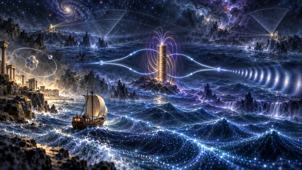
But when we try to carry this intuitively clear picture into quantum physics, the sea quickly becomes rough.
The Electron That Should Fall Into the Nucleus
One of the best-known historical signs that classical physics cannot simply be transferred into the atomic world is the problem of the electron moving around the nucleus.
If we imagine the electron as a small charged particle moving in a circular orbit, it has centripetal acceleration
From classical electrodynamics, we know that accelerated motion of charge leads to electromagnetic radiation.
In the nonrelativistic case, the Larmor formula gives the radiated power as
The electron should therefore continuously lose energy. Its orbit would shrink and, according to the classical picture, the atom would rapidly collapse.
But matter is stable.
The problem could not be solved by a small correction to classical electrodynamics. Something was wrong with the very picture of an electron circling the atomic nucleus like a planet around the Sun.
Bohr took the first radical step by postulating stationary states that do not radiate. De Broglie then associated wave properties with the electron, and Schrödinger later provided a mathematical theory in which the state of the electron is described by a wave function ψ(r,t).
For an energy eigenstate, it can be written as
The wave function has a time-dependent phase, but
is time-independent.
An electron in a stationary atomic state is therefore not a small ball accelerating along a classical orbit. Consequently, the Larmor formula cannot be applied directly to something that no longer possesses a classical trajectory.
This is one of the first major warnings when entering the domain of quantum physics: a mathematical or physical concept that works perfectly well in classical theory does not necessarily retain the same meaning once we cross into the quantum domain.
The Potential: Auxiliary Quantity or Something More?
A similar story exists in electromagnetism.
We describe electric and magnetic fields by the vectors E and B, but we may also introduce the scalar and vector potentials Φ and A.
Their relation to the fields is
and
In classical electromagnetism, it is natural to regard the potentials as elegant mathematical tools, while the fields E and B appear more directly physical because they are directly connected with measurable forces. The vector potential A therefore seems more abstract, but quantum mechanics seriously complicates this simple distinction.
A Short Note: What Is the Aharonov–Bohm Effect?
Imagine an electron interferometer in which the electron wave function is split into two coherent paths.
The paths enclose a region containing magnetic flux — for example, a very long solenoid — while the paths themselves pass through a region in which locally
Classically, we would expect the electron to experience no electromagnetic force along those paths.
Yet, after the two branches of the wave function are recombined, the interference pattern shifts.
The phase difference is
where ΦB is the magnetic flux enclosed by the paths.
The Aharonov–Bohm effect has been experimentally confirmed and represents one of the fundamental phenomena of quantum physics.
An important qualification is nevertheless required. This does not mean that the absolute phase of an isolated wave function is itself measurable. It is not. The physical effect comes from the relative phase between different coherent branches of the quantum state.
But the result remains profound: a quantity that in classical electromagnetism could easily be regarded mainly as a mathematical construct appears directly in a quantum phase that changes the outcome of an experiment.
Does the Electron “Feel” the Potential?
The textbook explanation of the Aharonov–Bohm effect often ends there.
The electron passes around the magnetic flux. Along its paths there is a nonzero vector potential. The two branches of the wave function acquire different phases and, when recombined, produce a shifted interference pattern.
But J. D. Franson, in his paper Covariance and the use of the Schrödinger equation in quantum field theory, formulates the problem differently.
He does not quantize only the electron in the interferometer while leaving the source of the magnetic field as a classical background.
In his formulation, the electron in the interferometer, the electromagnetic field, and the electrons producing the current in the magnetic-field source are all treated quantum mechanically.
This leads to a very interesting result.
The phase shift contains two symmetric terms:
The first term describes the interaction of the electron in the interferometer with the vector potential produced by the source.
The second describes the interaction of the electrons in the source with the vector potential produced by the electron in the interferometer.
In this formulation, both potentials are retarded.
This changes the intuitive picture.
The phase is no longer merely something the electron “picks up” while moving through an external potential. It becomes a property of the interaction of the entire quantum system.
In the Quasistatic Case, There Is No Problem
When the changes are sufficiently slow, that is, when retardation effects are negligible, the two contributions become equal.
Franson then obtains the standard expression
which is precisely the result experimentally observed in the magnetic Aharonov–Bohm effect.
Up to this point, his formulation does not contradict the known experiment.
The real question appears only when retardation can no longer be neglected.
Retarded Potentials and the Classical Picture of Causality
In classical electromagnetism, the vector potential at the point r and time t depends on the current at a distant point r′ at an earlier time.
Schematically,
The time
is called the retarded time.
Here the causal structure is completely clear: a change in the source cannot affect a distant point before light has had time to cross the distance between them.
But quantum field theory adds another layer.
The Feynman Propagator Is Not a Classical Electromagnetic Signal
In perturbative quantum field theory, the Feynman propagator appears.
It should not be imagined as the trajectory of a tiny particle — a virtual photon — simply flying from point A to point B.
The Feynman propagator represents a time-ordered correlation of the quantum field and, mathematically, does not have to vanish for spacelike-separated events.
Two events are spacelike separated if no signal traveling at the speed of light or slower can establish a causal connection between them. The order of such events can even be different in different inertial reference frames.
A nonzero Feynman propagator for such events does not by itself mean that we can send information faster than light.
Relativistic quantum theory introduces the requirement of microcausality: the appropriate local observables must commute when events are spacelike separated,
That is why we must distinguish three concepts that are often unjustifiably conflated in popular discussions:
Quantum-entangled states can show nonlocal correlations, but that does not imply the possibility of sending a message faster than light.
Franson’s Prediction: Only Half the Phase Shift
Franson considers a case in which the magnetic-field source and the interferometer are far enough apart that the electron passes through the interferometer before the electron’s retarded vector potential reaches the source.
Then, according to his derivation, the term
does not contribute to the phase during the relevant time interval.
Only the other part of the expression remains, and the author obtains
In other words,
— one half of the usual Aharonov–Bohm phase shift.
This is a bold prediction, but here it is essential to draw a clear line between theory and experiment.
The half phase shift caused by this retardation mechanism has not yet been experimentally confirmed.
Franson presents the result as a prediction and as a possible new experimental test of quantum electrodynamics, not as an experiment that has already been performed.
There are other experiments in which fractional or unusual Aharonov–Bohm periodicities appear, but their physical origin is different and they do not constitute confirmation of Franson’s retardation effect.
An Experiment That Is Not Entirely Impossible
Franson does not leave the problem at the level of a thought experiment alone.
He considers the possibility of using a SQUID interferometer with a response time of approximately one microsecond.
For
light travels approximately
The source and the interferometer would therefore have to be separated by hundreds of metres in order to eliminate the relevant retarded contribution from one side of the system during the measurement.
Such an experiment is clearly not simple, but neither is it a purely philosophical construction. In principle, it produces a measurable difference between Δφ and ½Δφ.
And that is precisely the difference between interpretative speculation and a physical hypothesis that can be subjected to experimental testing.
The More Uncomfortable Question: Causality
Franson then goes one step further.
He considers a time-dependent current in the magnetic-field source and chooses the geometry so that the change in current is spacelike separated from the final measurement of the electron in the interferometer.
In other words, the electromagnetic signal from the source cannot reach the interferometer before the measurement has already been completed.
Nevertheless, his derivation allows the change in current to influence the result of the interferometer.
If this represented a real physical effect, the problem would no longer be merely unusual quantum nonlocality, but a much more serious question of causality.
Why Does the Schrödinger Equation Appear Here?
The Schrödinger equation contains a privileged time coordinate:
It is therefore not manifestly Lorentz covariant.
That in itself is not new.
In standard relativistic scattering theory, the problem is handled by using asymptotic states for
where the interactions at the beginning and the end are effectively switched off.
The standard formalism then gives covariant results.
Franson, however, chooses a different problem: the measurement is performed at a finite time.
Because of the relativity of simultaneity, it is possible that in one reference frame a particular interaction has already ended at the moment of measurement, while in another the corresponding spacetime slice still includes part of the interaction.
This is precisely where the author locates the source of the problem.
Is a Local Observable Really Completely Local?
Perhaps the deepest part of the paper comes only after that.
The standard argument for microcausality starts from local field operators.
But Franson argues that, for a quantum-entangled system, the probability of detecting the electron in the interferometer cannot always be represented by an operator belonging only to a single point in space.
In his derivation, one must include a nonlocal product of operators describing both the electron and the distant source.
If this step is justified, the question is no longer:
“Does a virtual photon travel faster than light?”
That is probably the wrong question.
The more serious question is:
What exactly does a local observable mean when the quantum state of the system is spatially extended and quantum-entangled?
And even more deeply:
Does the locality of a measurement automatically imply the locality of the quantum state that determines the probability of that measurement?
Does This Mean Quantum Field Theory Is Incomplete?
Franson’s conclusion is radical.
He suggests that a formulation of quantum field theory based on Schrödinger time evolution or on equivalent Feynman path integrals may be incomplete for certain situations involving finite-time measurements and significant retardation.
That, however, is not the same as an established fact that QFT is acausal or wrong.
Relativistic quantum field theory is supported by an enormous body of extremely precise experimental confirmation.
If a particular construction produces an acausal result, at least two major possibilities remain open.
The first is the one emphasized by Franson: perhaps a genuine limitation of the standard formulation has been uncovered.
But there is also another possibility: perhaps the problem lies in the way the observable, the measurement, the source state, or the finite-time evolution of the system has been defined.
Before accepting such a strong conclusion as the fundamental incompleteness of QFT, these possibilities must be examined very carefully.
That is why experiment matters so much.
From the Non-Radiating Electron to the Question of What “Here” Means
Our voyage began with a simple classical question: if the electron moves with acceleration around the nucleus, why does it not radiate? The answer forced us to abandon the very idea of a classical orbit.
We then arrived at the Aharonov–Bohm effect, where the relative phase of a quantum state produces a measurable effect even when the electric and magnetic fields along the electron’s path are zero.
From there we moved into quantum field theory, where the Feynman propagator is not the same thing as a classical signal, and quantum nonlocality is not the same thing as superluminal communication.
And finally we arrived at Franson’s question: what happens when retardation, quantum nonlocality, and relativistic causality must all become part of the same experiment at the same time?
For now, there is no experimental confirmation of his predicted half Aharonov–Bohm phase shift. Perhaps an experiment will show that standard theory preserves causality perfectly well and that the problem lies in the way the calculation has been set up; or perhaps it will open a new question about the relationship between the quantum state, locality, and time. We do not yet know, and that is exactly where science becomes most interesting: not in the strangeness of the formula itself, but at the moment when highly successful mathematics begins to ask what we really mean by physical reality, locality, and causation.
We have charted routes on the maps of the Dirac Sea while sailing close to the shores of classical physics. But as we move away from those familiar coasts, the Dirac Sea becomes rougher, deeper, and more mysterious. 🌊⚛️
Leave a Reply